When it comes to Global Feature Descriptors (i.e feature vectors that quantifies the entire image), there are three major attributes to be considered - Color, Shape and Texture. All these three could be used separately or combined to quantify images. In this post, we will learn how to recognize texture in images. We will study a new type of global feature descriptor called Haralick Texture. Let’s jump right into it!
1
2
3
4
5
6
How to label and organize our own dataset?
What is Haralick Texture and how it is computed?
How to use Haralick Texture module in mahotas library?
How to recognize textures in images?
How to use Linear SVM to train and classify images?
How to make predictions using the created model on an unseen data?
What is a Texture?
Texture defines the consistency of patterns and colors in an object/image such as bricks, school uniforms, sand, rocks, grass etc. To classify objects in an image based on texture, we have to look for the consistent spread of patterns and colors in the object’s surface. Rough-Smooth, Hard-Soft, Fine-Coarse are some of the texture pairs one could think of, although there are many such pairs.
What is Haralick Texture?
Haralick Texture is used to quantify an image based on texture. It was invented by Haralick in 1973 and you can read about it in detail here. The fundamental concept involved in computing Haralick Texture features is the Gray Level Co-occurrence Matrix or GLCM.
What is GLCM?
Gray Level Co-occurrence matrix (GLCM) uses adjacency concept in images. The basic idea is that it looks for pairs of adjacent pixel values that occur in an image and keeps recording it over the entire image. Below figure explains how a GLCM is constructed.
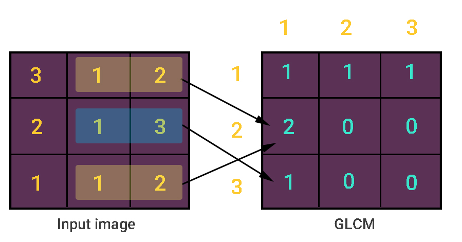
As you can see from the above image, gray-level pixel value 1 and 2 occurs twice in the image and hence GLCM records it as two. But pixel value 1 and 3 occurs only once in the image and thus GLCM records it as one. Of course, I have assumed the adjacency calculation only from left-to-right. Actually, there are four types of adjacency and hence four GLCM matrices are constructed for a single image. Four types of adjacency are as follows.
- Left-to-Right
- Top-to-Bottom
- Top Left-to-Bottom Right
- Top Right-to-Bottom Left
Haralick Texture Feature Vector
From the four GLCM matrices, 14 textural features are computed that are based on some statistical theory. All these 14 statistical features needs a separate blog post. So, you can read in detail about those here. Normally, the feature vector is taken to be of 13-dim as computing 14th dim might increase the computational time.
Implementing Texture Recognition
Ok, lets start with the code!
Actually, it will take just 10-15 minutes to complete our texture recognition system using OpenCV, Python, sklearn and mahotas provided we have the training dataset.
Note: In case if you don't have these packages installed, feel free to install these using my environment setup posts given below.
Import the necessary packages
1
2
3
4
5
6
import cv2
import numpy as np
import os
import glob
import mahotas as mt
from sklearn.svm import LinearSVC
Load the training dataset
1
2
3
4
5
6
7
# load the training dataset
train_path = "dataset/train"
train_names = os.listdir(train_path)

# empty list to hold feature vectors and train labels
train_features = []
train_labels = []
- Line 2 is the path to training dataset.
- Line 3 gets the class names of the training data.
- Line 6-7 are empty lists to hold feature vectors and labels.
Extract features function
1
2
3
4
5
6
7
def extract_features(image):
        # calculate haralick texture features for 4 types of adjacency
        textures = mt.features.haralick(image)

        # take the mean of it and return it
        ht_mean = textures.mean(axis=0)
        return ht_mean
- Line 1 is a function that takes an input image to compute haralick texture.
- Line 3 extracts the haralick features for all 4 types of adjacency.
- Line 6 finds the mean of all 4 types of GLCM.
- Line 7 returns the resulting feature vector for that image which describes the texture.
Extract features for all images
1
2
3
4
5
6
7
8
9
10
11
12
13
14
15
16
17
18
19
20
21
22
23
# loop over the training dataset
print "[STATUS] Started extracting haralick textures.."
for train_name in train_names:
        cur_path = train_path + "/" + train_name
        cur_label = train_name
        i = 1
        for file in glob.glob(cur_path + "/*.jpg"):
                print "Processing Image - {} in {}".format(i, cur_label)
                # read the training image
                image = cv2.imread(file)

                # convert the image to grayscale
                gray = cv2.cvtColor(image, cv2.COLOR_BGR2GRAY)

                # extract haralick texture from the image
                features = extract_features(gray)

                # append the feature vector and label
                train_features.append(features)
                train_labels.append(cur_label)

                # show loop update
                i += 1
- Line 4 loops over the training labels we have just included from training directory.
- Line 5 is the path to current image class directory.
- Line 6 holds the current image class label.
- Line 8 takes all the files with .jpg as the extension and loops through each file one by one.
- Line 11 reads the input image that corresponds to a file.
- Line 14 converts the image to grayscale.
- Line 17 extracts haralick features for the grayscale image.
- Line 20 appends the 13-dim feature vector to the training features list.
- Line 21 appends the class label to training classes list.
1
2
3
# have a look at the size of our feature vector and labels
print "Training features: {}".format(np.array(train_features).shape)
print "Training labels: {}".format(np.array(train_labels).shape)
Create the machine learning classifier
1
2
3
4
5
6
7
# create the classifier
print "[STATUS] Creating the classifier.."
clf_svm = LinearSVC(random_state=9)

# fit the training data and labels
print "[STATUS] Fitting data/label to model.."
clf_svm.fit(train_features, train_labels)
- Line 3 creates the Linear Support Vector Machine classifier.
- Line 7 fits the training features and labels to the classifier.
Test the classifier on testing data
1
2
3
4
5
6
7
8
9
10
11
12
13
14
15
16
17
18
19
20
21
# loop over the test images
test_path = "dataset/test"
for file in glob.glob(test_path + "/*.jpg"):
        # read the input image
        image = cv2.imread(file)

        # convert to grayscale
        gray = cv2.cvtColor(image, cv2.COLOR_BGR2GRAY)

        # extract haralick texture from the image
        features = extract_features(gray)

        # evaluate the model and predict label
        prediction = clf_svm.predict(features.reshape(1, -1))[0]

        # show the label
        cv2.putText(image, prediction, (20,30), cv2.FONT_HERSHEY_SIMPLEX, 1.0, (0,255,255), 3)

       # display the output image
       cv2.imshow("Test_Image", image)
       cv2.waitKey(0)
- Line 2 gets the testing data path.
- Line 3 takes all the files with the .jpg extension and loops through each file one by one.
- Line 5 reads the input image.
- Line 8 converts the input image into grayscale image.
- Line 11 extract haralick features from grayscale image.
- Line 14 predicts the output label for the test image.
- Line 17 displays the output class label for the test image.
- Finally, Line 20 displays the test image with predicted label.
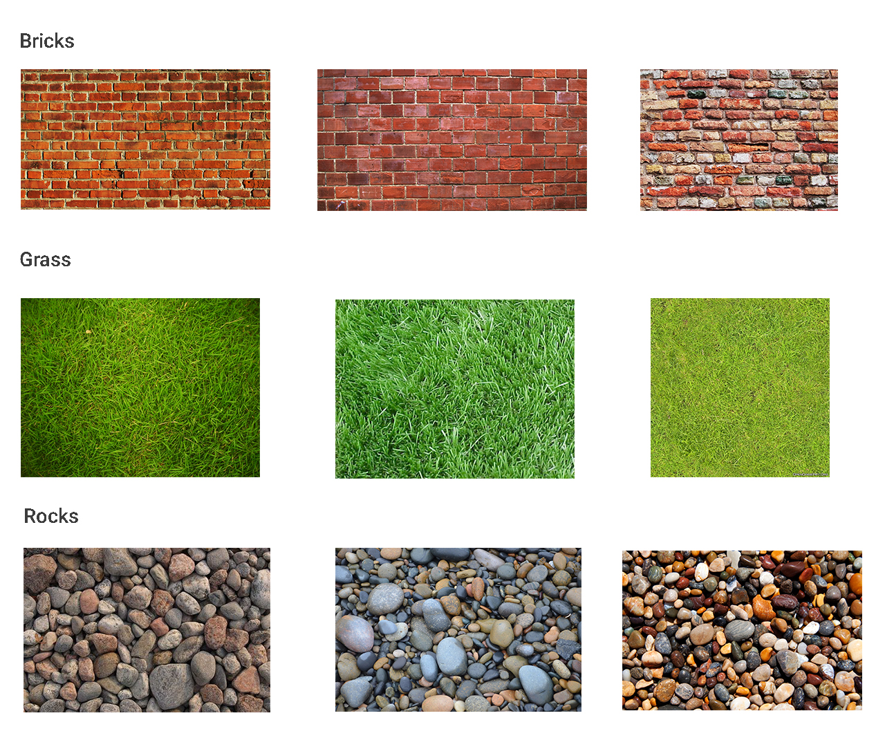
Training images
These are the images from which we train our machine learning classifier to learn texture features. You can collect the images of your choice and include it under a label. For example, “Grass” images are collected and stored inside a folder named “grass”. These images could either be taken from a simple google search (easy to do; but our model won’t generalize well) or from your own camera/smart-phone (which is indeed time-consuming, but our model could generalize well due to real-world images).
As a demonstration, I have included my own training and testing images. I took 3 classes of training images which holds 3 images per class. Training images with their corresponding class/label are shown below.
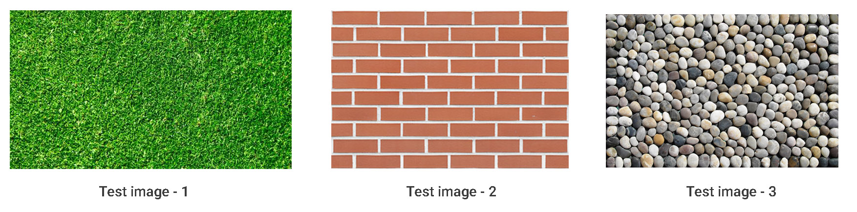
Testing images
These could be images or a video sequence from a smartphone/camera. We can test our model with this test data so that our model performs feature extraction on this text data and tries to come up with the best possible label/class.
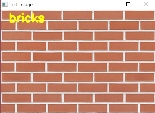
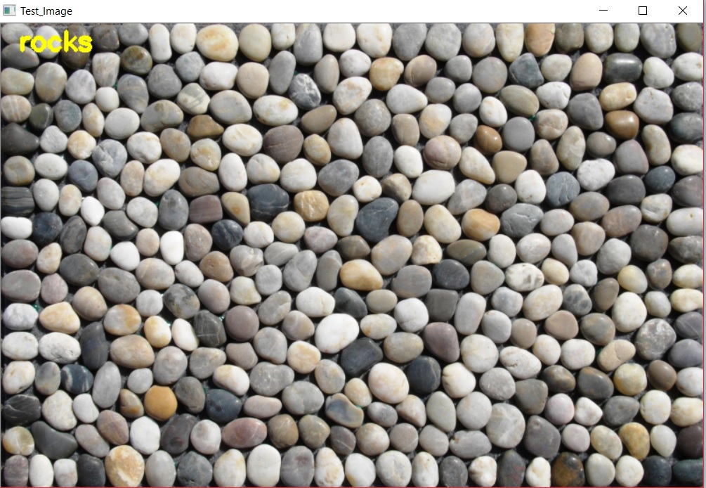
Some of the test images for which we need to predict the class/label are shown below.
Note: These test images won't have any label associated with them. Our model's purpose is to predict the best possible label/class for the image it sees.
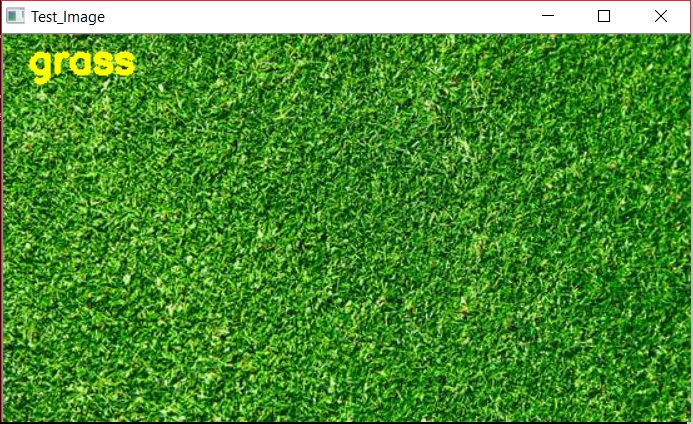
After running the code, our model was able to correctly predict the labels for the testing data as shown below.
Here is the entire code to build our texture recognition system.
1
2
3
4
5
6
7
8
9
10
11
12
13
14
15
16
17
18
19
20
21
22
23
24
25
26
27
28
29
30
31
32
33
34
35
36
37
38
39
40
41
42
43
44
45
46
47
48
49
50
51
52
53
54
55
56
57
58
59
60
61
62
63
64
65
66
67
68
69
70
71
72
73
74
75
76
77
78
79
80
81
82
83
import cv2
import numpy as np
import os
import glob
import mahotas as mt
from sklearn.svm import LinearSVC

# function to extract haralick textures from an image
def extract_features(image):
	# calculate haralick texture features for 4 types of adjacency
	textures = mt.features.haralick(image)

	# take the mean of it and return it
	ht_mean  = textures.mean(axis=0)
	return ht_mean

# load the training dataset
train_path  = "dataset/train"
train_names = os.listdir(train_path)

# empty list to hold feature vectors and train labels
train_features = []
train_labels   = []

# loop over the training dataset
print "[STATUS] Started extracting haralick textures.."
for train_name in train_names:
	cur_path = train_path + "/" + train_name
	cur_label = train_name
	i = 1

	for file in glob.glob(cur_path + "/*.jpg"):
		print "Processing Image - {} in {}".format(i, cur_label)
		# read the training image
		image = cv2.imread(file)

		# convert the image to grayscale
		gray = cv2.cvtColor(image, cv2.COLOR_BGR2GRAY)

		# extract haralick texture from the image
		features = extract_features(gray)

		# append the feature vector and label
		train_features.append(features)
		train_labels.append(cur_label)

		# show loop update
		i += 1

# have a look at the size of our feature vector and labels
print "Training features: {}".format(np.array(train_features).shape)
print "Training labels: {}".format(np.array(train_labels).shape)

# create the classifier
print "[STATUS] Creating the classifier.."
clf_svm = LinearSVC(random_state=9)

# fit the training data and labels
print "[STATUS] Fitting data/label to model.."
clf_svm.fit(train_features, train_labels)

# loop over the test images
test_path = "dataset/test"
for file in glob.glob(test_path + "/*.jpg"):
	# read the input image
	image = cv2.imread(file)

	# convert to grayscale
	gray = cv2.cvtColor(image, cv2.COLOR_BGR2GRAY)

	# extract haralick texture from the image
	features = extract_features(gray)

	# evaluate the model and predict label
	prediction = clf_svm.predict(features.reshape(1, -1))[0]

	# show the label
	cv2.putText(image, prediction, (20,30), cv2.FONT_HERSHEY_SIMPLEX, 1.0, (0,255,255), 3)
	print "Prediction - {}".format(prediction)

	# display the output image
	cv2.imshow("Test_Image", image)
	cv2.waitKey(0)
1
2
3
4
5
6
7
8
9
10
11
12
13
14
15
16
17
[STATUS] Started extracting haralick textures..
Processing Image - 1 in bricks
Processing Image - 2 in bricks
Processing Image - 3 in bricks
Processing Image - 1 in grass
Processing Image - 2 in grass
Processing Image - 3 in grass
Processing Image - 1 in rocks
Processing Image - 2 in rocks
Processing Image - 3 in rocks
Training features: (9, 13)
Training labels: (9,)
[STATUS] Creating the classifier..
[STATUS] Fitting data/label to model..
Prediction - grass
Prediction - bricks
Prediction - rocks
If you copy-paste the above code in any of your directory and run python train_test.py, you will get the following results.
Thus, we have implemented our very own Texture Recognition system using Haralick Textures, Python and OpenCV.
In case if you found something useful to add to this article or you found a bug in the code or would like to improve some points mentioned, feel free to write it down in the comments. Hope you found something useful here.