Before understanding the math behind a Deep Neural Network and implementing it in code, it is better to get a mindset of how Logistic Regression algorithm could be modelled as a simple Neural Network that actually learns from data. Implementing AI algorithms from scratch gives you that “ahha” moment and confidence to build your own algorithms in future.
Update: As Python2 faces end of life, the below code only supports Python3.
1
2
3
4
How to convert an image into a vector?
How to preprocess an existing image dataset to do Deep Learning?
How to represent images and labels as numpy arrays?
How to use just one for-loop to train a logistic regression model?
A look at what we will be building at the end of this tutorial is shown below. A binary classifier that will classify an image as either airplane or bike.
Prerequisites
Before reading this tutorial, you must have some basic understanding of the following.
Image as a vector
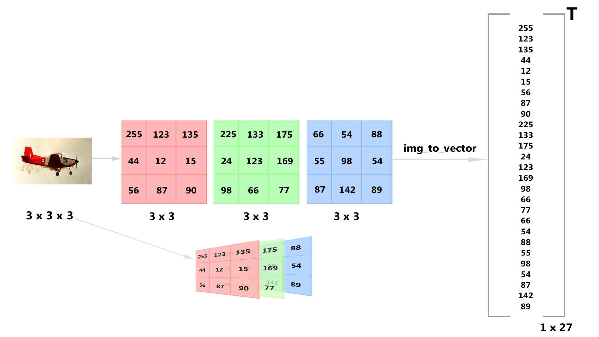
The input to the logistic regression model is an image. An image is a three-dimensional matrix that holds pixel intensity values of Red, Green and Blue channels. In Deep Learning, what we do first is that we convert this image (3d-matrix) to a 1d-matrix (also called as a vector).
For example, if our image is of dimension [640, 480, 3] where 640 is the width, 480 is the height and 3 is the number of channels, then the flattened version of the image or 1-d representation of the image will be [1, 921600].
Notice that in the above vector dimension, we represent the image as a row vector having 921600 columns.
To better understand this, look at the image below.
Dataset
We will use the CALTECH-101 dataset which has images belonging to 101 categories such as airplane, bike, elephant etc. As we are dealing with a binary classification problem, we will specifically use images from two categories airplane and bike.
Download this dataset and make sure you follow the below folder structure.
1
2
3
4
5
6
7
8
9
10
11
12
13
14
15
16
17
18
19
20
21
22
23
24
25
|--logistic-regression
|--|--dataset
|--|--|--train
|--|--|--|--airplane
|--|--|--|--|--image_1.jpg
|--|--|--|--|--image_2.jpg
|--|--|--|--|--....
|--|--|--|--|--image_750.jpg
|--|--|--|--bike
|--|--|--|--|--image_1.jpg
|--|--|--|--|--image_2.jpg
|--|--|--|--|--....
|--|--|--|--|--image_750.jpg
|--|--|--test
|--|--|--|--airplane
|--|--|--|--|--image_1.jpg
|--|--|--|--|--image_2.jpg
|--|--|--|--|--....
|--|--|--|--|--image_50.jpg
|--|--|--|--bike
|--|--|--|--|--image_1.jpg
|--|--|--|--|--image_2.jpg
|--|--|--|--|--....
|--|--|--|--|--image_50.jpg
|--|--train.py
Inside the train folder, you need to create two sub-folders namely airplane and bike. You have to manually copy 750 images from airplane folder in “CALTECH-101” dataset to our airplane folder. Similarly, you have to manually copy 750 images from motorbikes folder in “CALTECH-101” dataset to our bike folder.
Inside the test folder, you have to do the same process, but now, you will be having 50 images in airplane and 50 images in bike.
Before starting anything, make sure you have the following number of images in each folder.
- dataset -> train -> airplane -> 750 images
- dataset -> train -> bike -> 750 images
- dataset -> test -> airplane -> 50 images
- dataset -> test -> bike -> 50 images
Prepare the dataset
Let’s fix the input image size with dimensions \([64, 64, 3]\), meaning \(64\) is the width and height with \(3\) channels. The flattened vector will then have dimension \([1, 12288]\). We will also need to know the total number of training images that we are going to use so that we can build an empty numpy array with that dimension and then fill it up after flattening every image. In our case, total number of train images num_train_images = \(1500\) and total number of test images num_test_images = \(100\).
We need to define four numpy arrays filled with zeros.
- Array of dimension \([12288, 1500]\) to hold our train images.
- Array of dimension \([12288, 100]\) to hold our test images.
- Array of dimension \([1, 1500]\) to hold our train labels.
- Array of dimension \([1, 100]\) to hold our test labels.
For each image in the dataset:
- Convert the image into a matrix of fixed size using load_img() in Keras - \([64, 64, 3]\).
- Convert the image into a row vector using flatten() in NumPy - \([12288,]\)
- Expand the dimensions of the above vector using np.expand_dims() in NumPy - \([1, 12288]\)
- Concatenate this vector to a numpy array train_x of dimension \([12288, 1500]\).
- Concatenate this vector’s label to a numpy array train_y of dimension \([1, 1500]\).
We need to perform the above procedure for test data to get test_x and test_y.
We then standardize train_x and test_x by dividing each pixel intensity value by 255. This is because normalizing the image matrix makes our learning algorithm better.
Also, we will assign “0” as the label to airplane and “1” as the label to bike. This is very important as computers work only with numbers.
Finally, we can save all our four numpy arrays locally using h5py library.
Below is the code snippet to do all the above steps before building our logistic regression neural network model.
1
2
3
4
5
6
7
8
9
10
11
12
13
14
15
16
17
18
19
20
21
22
23
24
25
26
27
28
29
30
31
32
33
34
35
36
37
38
39
40
41
42
43
44
45
46
47
48
49
50
51
52
53
54
55
56
57
58
59
60
61
62
63
64
65
66
67
68
69
70
71
72
73
74
75
76
77
78
79
80
81
82
83
84
85
86
87
88
89
#-------------------
# organize imports
#-------------------
import numpy as np
import os
import h5py
import glob
import cv2
from keras.preprocessing import image

#------------------------
# dataset pre-processing
#------------------------
train_path   = "G:\\workspace\\machine-intelligence\\deep-learning\\logistic-regression\\dataset\\train"
test_path    = "G:\\workspace\\machine-intelligence\\deep-learning\\logistic-regression\\dataset\\test"
train_labels = os.listdir(train_path)
test_labels  = os.listdir(test_path)

# tunable parameters
image_size       = (64, 64)
num_train_images = 1500
num_test_images  = 100
num_channels     = 3

# train_x dimension = {(64*64*3), 1500}
# train_y dimension = {1, 1500}
# test_x dimension  = {(64*64*3), 100}
# test_y dimension  = {1, 100}
train_x = np.zeros(((image_size[0]*image_size[1]*num_channels), num_train_images))
train_y = np.zeros((1, num_train_images))
test_x  = np.zeros(((image_size[0]*image_size[1]*num_channels), num_test_images))
test_y  = np.zeros((1, num_test_images))

#----------------
# TRAIN dataset
#----------------
count = 0
num_label = 0
for i, label in enumerate(train_labels):
	cur_path = train_path + "\\" + label
	for image_path in glob.glob(cur_path + "/*.jpg"):
		img = image.load_img(image_path, target_size=image_size)
		x   = image.img_to_array(img)
		x   = x.flatten()
		x   = np.expand_dims(x, axis=0)
		train_x[:,count] = x
		train_y[:,count] = num_label
		count += 1
	num_label += 1

#--------------
# TEST dataset
#--------------
count = 0
num_label = 0
for i, label in enumerate(test_labels):
	cur_path = test_path + "\\" + label
	for image_path in glob.glob(cur_path + "/*.jpg"):
		img = image.load_img(image_path, target_size=image_size)
		x   = image.img_to_array(img)
		x   = x.flatten()
		x   = np.expand_dims(x, axis=0)
		test_x[:,count] = x
		test_y[:,count] = num_label
		count += 1
	num_label += 1

#------------------
# standardization
#------------------
train_x = train_x/255.
test_x  = test_x/255.

print("train_labels : " + str(train_labels))
print("train_x shape: " + str(train_x.shape))
print("train_y shape: " + str(train_y.shape))
print("test_x shape : " + str(test_x.shape))
print("test_y shape : " + str(test_y.shape))

#-----------------
# save using h5py
#-----------------
h5_train = h5py.File("train_x.h5", 'w')
h5_train.create_dataset("data_train", data=np.array(train_x))
h5_train.close()

h5_test = h5py.File("test_x.h5", 'w')
h5_test.create_dataset("data_test", data=np.array(test_x))
h5_test.close()
1
2
3
4
5
train_labels : ['airplane', 'bike']
train_x shape: (12288, 1500)
train_y shape: (1, 1500)
test_x shape : (12288, 100)
test_y shape : (1, 100)
Logistic Regression pipeline
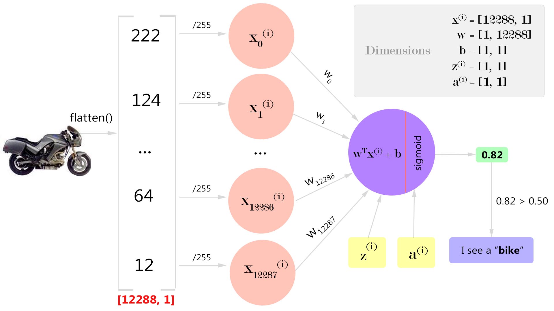
By looking at the above figure, the problem that we are going to solve is this -
Given an input image, our model must be able to figure out the label by telling whether it is an airplane or a bike.
A simple neuron
An artificial neuron (shown as purple circle in Figure 3) is a biologically inspired representation of a neuron inside human brain. Similar to a neuron in human brain, an artificial neuron accepts inputs from some other neurons and fires a value to the next set of artificial neurons. Inside a single neuron, two computations are performed.
- Weighted sum
- Activation
Weighted sum
Every input value \(x_{(i)}\) to an artificial neuron has a weight \(w_{(i)}\) associated with it which tells about the relative importance of that input with other inputs. Each weight \(w_{(i)}\) is multiplied with its corresponding input \(x_{(i)}\) and gets summed up to produce a single value \(z\).
Activation
After computing the weighted sum \(z\), an activation function \(a = g(z)\) is applied to this weighted sum \(z\). Activation function is a simple mathematical transformation of an input value to an output value by introducing a non-linearity. This is necessary because real-world inputs are non-linear and we need our neural network to learn this non-linearity somehow.
Logistic Regression concept
- Initialize the weights w and biases b to random values (say 0 or using random distribution).
- Foreach training sample in the dataset -
- Calculate the output value \(a^{(i)}\) for an input sample \(x^{(i)}\).
- First: find out the weighted sum \(z^{(i)}\).
- Second: compute the activation value \(a^{(i)}\) = \(y’^{(i)}\) = \(g(z^{(i)})\) for the weighted sum \(z^{(i)}\).
- As we know the true label for this input training sample \(y^{(i)}\), we use that to find the loss \(L(a^{(i)},y^{(i)})\).
- Calculate the output value \(a^{(i)}\) for an input sample \(x^{(i)}\).
- Calculate the cost function \(J\) which is the sum of all losses divided by the number of training examples \(m\) i.e., \(\frac{1}{m}\sum_{i=1}^m L(a^{(i)},y^{(i)})\).
- To minimize the cost function, compute the gradients for parameters \(\frac{dJ}{dw}\) and \(\frac{dJ}{db}\) using chain rule of calculus.
- Use gradient descent to update the parameters w and b.
- Perform the above procedure till the cost function becomes minimum.
Vectorization
One interesting thing in the above algorithm is that we will not be using the for loop (2nd point) in code; rather we will use vectorization offered by numpy to speed up computations in an efficient way.
After successfully pre-processing the dataset, please look at the below image to visually understand how the dimensions of our numpy arrays look like.
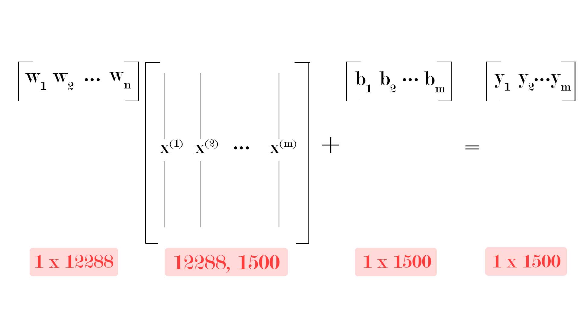
As you can see, the weights array has a dimension of shape \([1, 12288]\) and biases array has a dimension of shape \([1, 1500]\). But you will see that we will be initializing bias as a single value. A concept called broadcasting automatically applies the single b value to the matrix of shape \([1, 1500]\).
Gradient Descent
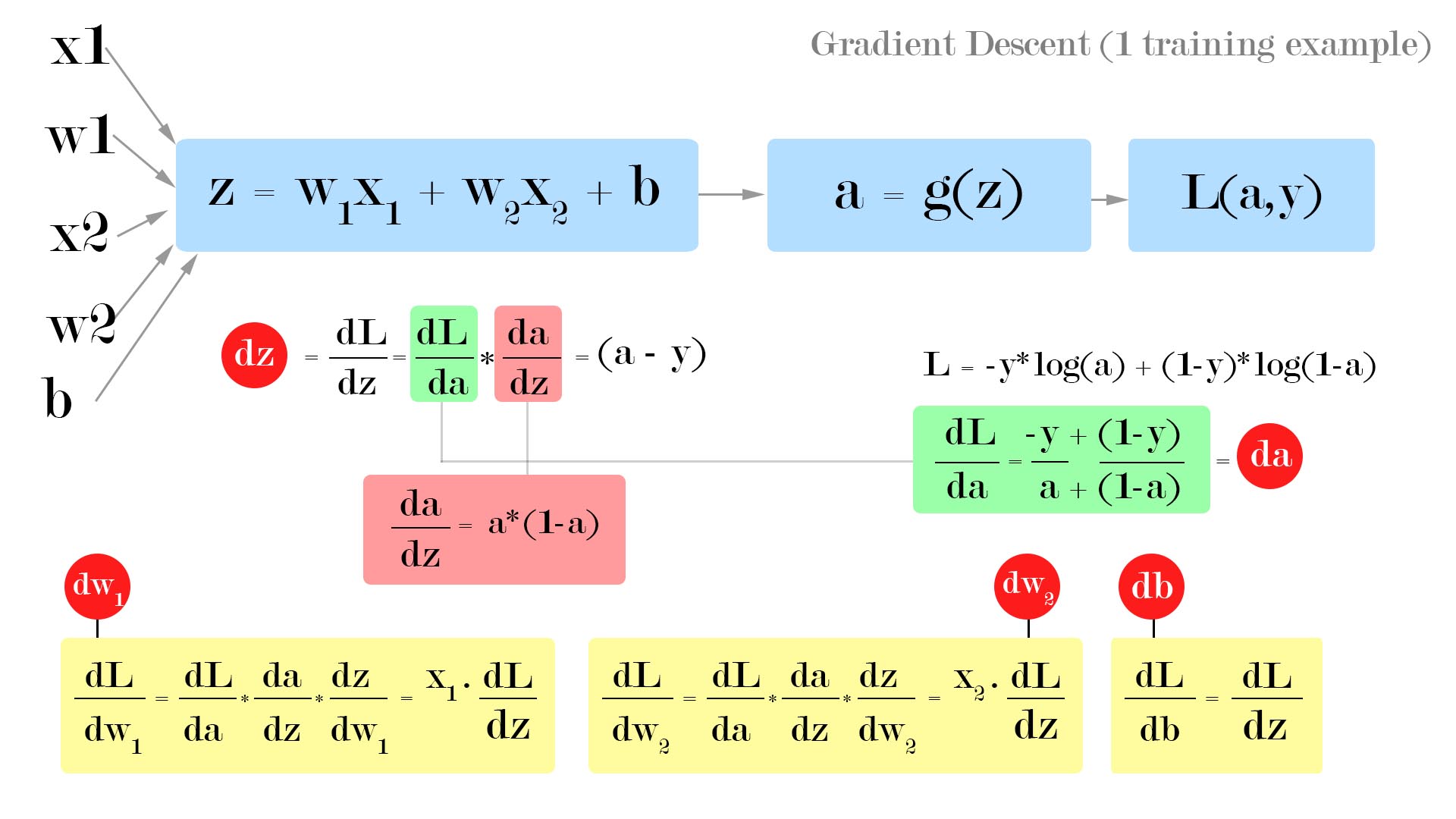
The above figure shows us how to visualize forward propagation and backpropagation as a computation graph for one training example.
- Forward propagation (for a single training example)
- Calculate the weighted sum \(z = w_1x_1 + w_2x_2 + b\).
- Calculate the activation \(a = \sigma(z)\).
- Compute the loss \(L(a,y) = -ylog(a)+(1-y)log(1-a)\).
- Backpropagation (for a single training example)
- Compute the derivatives of parameters \(\frac{dL}{dw1}\), \(\frac{dL}{dw2}\) and \(\frac{dL}{db}\) using \(\frac{dL}{da}\) and \(\frac{dL}{dz}\).
- Use update rule to update the parameters.
- \(w1 = w1 -\alpha \frac{dL}{dw1}\)
- \(w2 = w2 -\alpha \frac{dL}{dw2}\)
- \(b = b -\alpha \frac{dL}{db}\)
In code, we will be denoting \(\frac{dL}{dw1}\) as dw1, \(\frac{dL}{dw2}\) as dw2, \(\frac{dL}{db}\) as db, \(\frac{dL}{da}\) as da and \(\frac{dL}{dz}\) as dz.
But in our problem we don’t just have 1 training example, rather \(m\) training examples. This is where cost function \(J\) comes into picture. So, we calculate losses for all the training examples, sum it up and divide by the number of training examples \(m\).
Mathematical equations
There are 7 mathematical equations to build a logistic regression model with a neural network mindset. Everything else is vectorization. So, the core concept in building neural networks is to understand these equations thoroughly.
Weighted Sum of \(i^{th}\) training example
Activation of \(i^{th}\) training example (using sigmoid)
Loss function of \(i^{th}\) training example
Cost function for all training examples
Gradient Descent w.r.t cost function, weights and bias
Parameters update rule
Math to Code
We will be using the below functions to create and train our logistic regression neural network model.
1. sigmoid()
- Input - a number or a numpy array.
- Output - sigmoid of the number or the numpy array.
1
2
def sigmoid(z):
	return (1/(1+np.exp(-z)))
2. init_params()
- Input - dimension for weights (every value in an image’s vector has a weight associated with it).
- Output - weight vector w and bias b
1
2
3
4
def init_params(dimension):
	w = np.zeros((dimension, 1))
	b = 0
	return w, b
3. propagate()
- Input - weight vector w, bias b, image matrix X and label vector Y.
- Output - gradients dw, db and cost function costs for every 100 iterations.
1
2
3
4
5
6
7
8
9
10
11
12
13
14
15
16
17
18
def propagate(w, b, X, Y):
	# num of training samples
	m = X.shape[1]

	# forward pass
	A    = sigmoid(np.dot(w.T,X) + b)
	cost = (-1/m)*(np.sum(np.multiply(Y,np.log(A)) + np.multiply((1-Y),np.log(1-A))))

	# back propagation
	dw = (1/m)*(np.dot(X, (A-Y).T))
	db = (1/m)*(np.sum(A-Y))

	cost = np.squeeze(cost)

	# gradient dictionary
	grads = {"dw": dw, "db": db}

	return grads, cost
4. optimize()
- Input - weight vector w, bias b, image matrix X, label vector Y, number of iterations for gradient descent epochs and learning rate lr.
- Output - parameter dictionary params holding updated w and b, gradient dictionary grads holding dw and db, and list of cost function costs after every 100 iterations.
1
2
3
4
5
6
7
8
9
10
11
12
13
14
15
16
17
18
19
20
21
22
23
24
25
def optimize(w, b, X, Y, epochs, lr):
	costs = []
	for i in range(epochs):
		# calculate gradients
		grads, cost = propagate(w, b, X, Y)

		# get gradients
		dw = grads["dw"]
		db = grads["db"]

		# update rule
		w = w - (lr*dw)
		b = b - (lr*db)

		if i % 100 == 0:
			costs.append(cost)
			print("cost after %i epochs: %f" %(i, cost))

	# param dict
	params = {"w": w, "b": b}

	# gradient dict
	grads  = {"dw": dw, "db": db}

	return params, grads, costs
5. predict()
- Input - updated parameters w, b and image matrix X.
- Output - predicted labels Y_predict for the image matrix X.
1
2
3
4
5
6
7
8
9
10
11
12
13
14
def predict(w, b, X):
	m = X.shape[1]
	Y_predict = np.zeros((1,m))
	w = w.reshape(X.shape[0], 1)

	A = sigmoid(np.dot(w.T, X) + b)

	for i in range(A.shape[1]):
		if A[0, i] <= 0.5:
			Y_predict[0, i] = 0
		else:
			Y_predict[0,i]  = 1

	return Y_predict
6. predict_image()
- Input - updated parameters w, b and a single image vector X.
- Output - predicted label Y_predict for the single image vector X.
1
2
3
4
5
6
7
8
9
10
11
def predict_image(w, b, X):
	Y_predict = None
	w = w.reshape(X.shape[0], 1)
	A = sigmoid(np.dot(w.T, X) + b)
	for i in range(A.shape[1]):
		if A[0, i] <= 0.5:
			Y_predict = 0
		else:
			Y_predict = 1

	return Y_predict
Fitting it all together
We will use all the above functions into a main function named model().
- Input - Training image matrix X_train, Training image labels Y_train, Testing image matrix X_test, Test image labels Y_test, number of iterations for gradient descent epochs and learning rate lr.
- Output - Logistic regression model dictionary having the parameters (w,b), predictions, costs, learning rate, epochs.
1
2
3
4
5
6
7
8
9
10
11
12
13
14
15
16
17
18
19
20
21
22
def model(X_train, Y_train, X_test, Y_test, epochs, lr):
	w, b = init_params(X_train.shape[0])
	params, grads, costs = optimize(w, b, X_train, Y_train, epochs, lr)

	w = params["w"]
	b = params["b"]

	Y_predict_train = predict(w, b, X_train)
	Y_predict_test  = predict(w, b, X_test)

	print("train_accuracy: {} %".format(100-np.mean(np.abs(Y_predict_train - Y_train)) * 100))
	print("test_accuracy : {} %".format(100-np.mean(np.abs(Y_predict_test  - Y_test)) * 100))

	log_reg_model = {"costs": costs,
				     "Y_predict_test": Y_predict_test,
					 "Y_predict_train" : Y_predict_train,
					 "w" : w,
					 "b" : b,
					 "learning_rate" : lr,
					 "epochs": epochs}

	return log_reg_model
Training the model
Finally, we can train our model using the below code. This produces the train accuracy and test accuracy for the dataset.
1
2
# activate the logistic regression model
myModel = model(train_x, train_y, test_x, test_y, epochs, lr)
1
2
3
4
5
6
7
8
9
10
11
12
13
14
15
16
17
18
19
20
21
22
23
24
25
26
27
28
Using TensorFlow backend.
train_labels : ['airplane', 'bike']
train_x shape: (12288, 1500)
train_y shape: (1, 1500)
test_x shape : (12288, 101)
test_y shape : (1, 101)
cost after 0 epochs: 0.693147
cost after 100 epochs: 0.136297
cost after 200 epochs: 0.092398
cost after 300 epochs: 0.076973
cost after 400 epochs: 0.067062
cost after 500 epochs: 0.059735
cost after 600 epochs: 0.053994
cost after 700 epochs: 0.049335
cost after 800 epochs: 0.045456
cost after 900 epochs: 0.042167
cost after 1000 epochs: 0.039335
cost after 1100 epochs: 0.036868
cost after 1200 epochs: 0.034697
cost after 1300 epochs: 0.032769
cost after 1400 epochs: 0.031045
cost after 1500 epochs: 0.029493
cost after 1600 epochs: 0.028088
cost after 1700 epochs: 0.026810
cost after 1800 epochs: 0.025642
cost after 1900 epochs: 0.024570
train_accuracy: 99.66666666666667 %
test_accuracy : 100.0 %
Testing the trained model (optional)
We can use OpenCV to visualize our model’s performance on test dataset. Below code snipped takes it four images, our model predicts the label for these four images and displays it on the screen.
1
2
3
4
5
6
7
8
9
10
11
12
13
14
15
16
17
18
19
20
21
22
23
24
25
26
test_img_paths = ["G:\\workspace\\machine-intelligence\\deep-learning\\logistic-regression\\dataset\\test\\airplane\\image_0723.jpg",
                  "G:\\workspace\\machine-intelligence\\deep-learning\\logistic-regression\\dataset\\test\\airplane\\image_0713.jpg",
                  "G:\\workspace\\machine-intelligence\\deep-learning\\logistic-regression\\dataset\\test\\bike\\image_0782.jpg",
                  "G:\\workspace\\machine-intelligence\\deep-learning\\logistic-regression\\dataset\\test\\bike\\image_0799.jpg",
                  "G:\\workspace\\machine-intelligence\\deep-learning\\logistic-regression\\dataset\\test\\bike\\test_1.jpg"]

for test_img_path in test_img_paths:
	img_to_show    = cv2.imread(test_img_path, -1)
	img            = image.load_img(test_img_path, target_size=image_size)
	x              = image.img_to_array(img)
	x              = x.flatten()
	x              = np.expand_dims(x, axis=1)
	predict        = predict_image(myModel["w"], myModel["b"], x)
	predict_label  = ""

	if predict == 0:
		predict_label = "airplane"
	else:
		predict_label = "bike"

	# display the test image and the predicted label
	cv2.putText(img_to_show, predict_label, (30,20), cv2.FONT_HERSHEY_SIMPLEX, 1, (0,0,255), 2)
	cv2.imshow("test_image", img_to_show)
	key = cv2.waitKey(0) & 0xFF
	if (key == 27):
		cv2.destroyAllWindows()
Resources
In case if you found something useful to add to this article or you found a bug in the code or would like to improve some points mentioned, feel free to write it down in the comments. Hope you found something useful here.