The ability of a machine learning model to classify or label an image into its respective class with the help of learned features from hundreds of images is called as Image Classification.
Note: This tutorial is specific to Windows environment. Please modify code accordingly to work in other environments such as Linux and Max OS.
This is typically a supervised learning problem where we humans must provide training data (set of images along with its labels) to the machine learning model so that it learns how to discriminate each image (by learning the pattern behind each image) with respect to its label.
Update (03/07/2019): As Python2 faces end of life, the below code only supports Python3.
In this post, we will look into one such image classification problem namely Flower Species Recognition, which is a hard problem because there are millions of flower species around the world. As we know machine learning is all about learning from past data, we need huge dataset of flower images to perform real-time flower species recognition. Without worrying too much on real-time flower recognition, we will learn how to perform a simple image classification task using computer vision and machine learning algorithms with the help of Python.
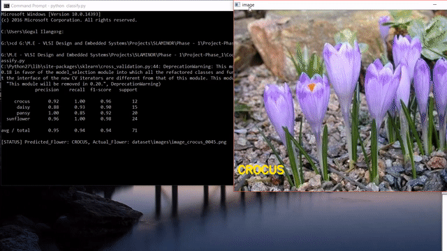
A short clip of what we will be making at the end of the tutorial 😊
Update: After reading this post, you could look into my post on how to use state-of-the-art pretrained deep learning models such as Inception-V3, Xception, VGG16, VGG19, ResNet50, InceptionResNetv2 and MobileNet to this flower species recognition problem.
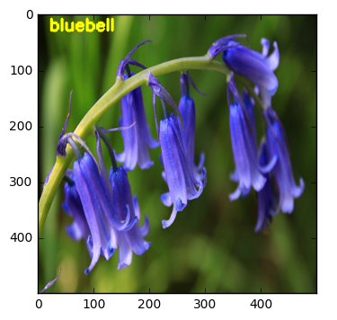
Image taken from here
Project Idea
What if
- You build an intelligent system that was trained with massive dataset of flower/plant images.
- Your system predicts the label/class of the flower/plant using Computer Vision techniques and Machine Learning algorithms.
- Your system searches the web for all the flower/plant related data after predicting the label/class of the captured image.
- Your system helps gardeners and farmers to increase their productivity and yield with the help of automating tasks in garden/farm.
- Your system applies the recent technological advancements such as Internet of Things (IoT) and Machine Learning in the agricultural domain.
- You build such a system for your home or your garden to monitor your plants using a Raspberry Pi.
All the above scenarios need a common task to be done at the first place - Image Classification.
Yeah! It is classifying a flower/plant into it’s corresponding class or category. For example, when our awesome intelligent assistant looks into a Sunflower image, it must label or classify it as a “Sunflower”.
Classification Problem
Plant or Flower Species Classification is one of the most challenging and difficult problems in Computer Vision due to a variety of reasons.
Availability of plant/flower dataset
Collecting plant/flower dataset is a time-consuming task. You can visit the links provided at the bottom of this post where I have collected all the publicly available plant/flower datasets around the world. Although traning a machine with these dataset might help in some scenerios, there are still more problems to be solved.
Millions of plant/flower species around the world
This is something very interesting to look from a machine learning point of view. When I looked at the numbers in this link, I was frightened. Because, to accomodate every such species, we need to train our model with such large number of images with its labels. We are talking about 6 digit class labels here for which we need tremendous computing power (GPU farms).
High inter-class as well as intra-class variation
What we mean here is that “Sunflower” might be looking similar to a “Daffodil” in terms of color. This becomes an inter-class variation problem. Similarly, sometimes a single “Sunflower” image might have differences within it’s class itself, which boils down to intra-class variation problem.
Fine-grained classification problem
It means our model must not look into the image or video sequence and find “Oh yes! there is a flower in this image”. It means our model must tell “Yeah! I found a flower in this image and I can tell you it’s a tulip”.
Segmentation, View-point, Occlusion, Illumination and the list goes on..
Segmenting the plant/flower region from an image is a challenging task. This is because we might need to remove the unwanted background and take only the foreground object (plant/flower) which is again a difficult thing due to the shape of plant/flower.
Image taken from here
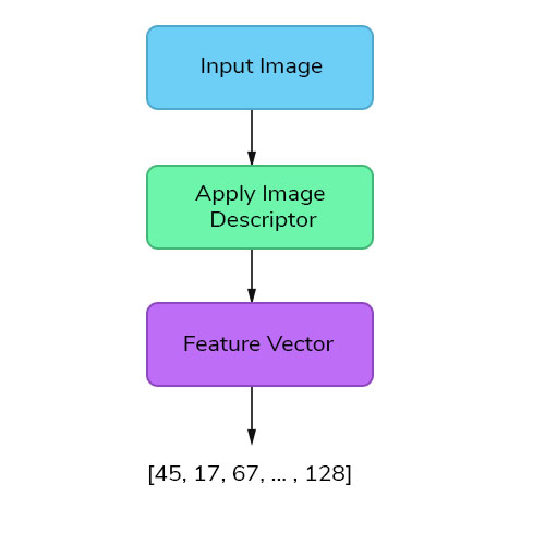
Feature Extraction
Features are the information or list of numbers that are extracted from an image. These are real-valued numbers (integers, float or binary). There are a wider range of feature extraction algorithms in Computer Vision.
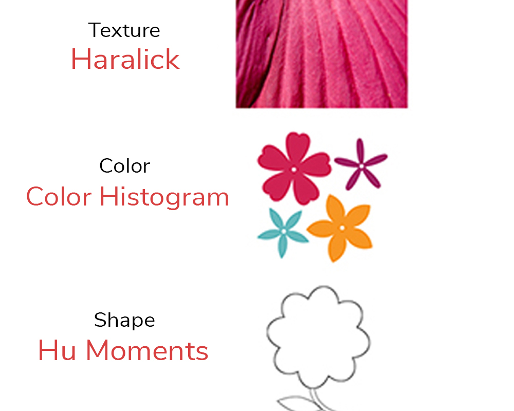
When deciding about the features that could quantify plants and flowers, we could possibly think of Color, Texture and Shape as the primary ones. This is an obvious choice to globally quantify and represent the plant or flower image.
But this approach is less likely to produce good results, if we choose only one feature vector, as these species have many attributes in common like sunflower will be similar to daffodil in terms of color and so on. So, we need to quantify the image by combining different feature descriptors so that it describes the image more effectively.
Global Feature Descriptors
These are the feature descriptors that quantifies an image globally. These don’t have the concept of interest points and thus, takes in the entire image for processing. Some of the commonly used global feature descriptors are
- Color - Color Channel Statistics (Mean, Standard Deviation) and Color Histogram
- Shape - Hu Moments, Zernike Moments
- Texture - Haralick Texture, Local Binary Patterns (LBP)
- Others - Histogram of Oriented Gradients (HOG), Threshold Adjancency Statistics (TAS)
Local Feature Descriptors
These are the feature descriptors that quantifies local regions of an image. Interest points are determined in the entire image and image patches/regions surrounding those interest points are considered for analysis. Some of the commonly used local feature descriptors are
- SIFT (Scale Invariant Feature Transform)
- SURF (Speeded Up Robust Features)
- ORB (Oriented Fast and Rotated BRIEF)
- BRIEF (Binary Robust Independed Elementary Features)
Combining Global Features
There are two popular ways to combine these feature vectors.
- For global feature vectors, we just concatenate each feature vector to form a single global feature vector. This is the approach we will be using in this tutorial.
- For local feature vectors as well as combination of global and local feature vectors, we need something called as Bag of Visual Words (BOVW). This approach is not discussed in this tutorial, but there are lots of resources to learn this technique. Normally, it uses Vocabulory builder, K-Means clustering, Linear SVM, and Td-Idf vectorization.
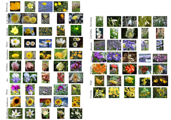
FLOWERS-17 dataset
We will use the FLOWER17 dataset provided by the University of Oxford, Visual Geometry group. This dataset is a highly challenging dataset with 17 classes of flower species, each having 80 images. So, totally we have 1360 images to train our model. For more information about the dataset and to download it, kindly visit this link.
Organizing Dataset
The folder structure for this example is given below.
folder structure
1
2
3
4
5
6
7
8
9
10
11
12
13
14
15
16
17
18
19
20
|--image-classification (folder)
|--|--dataset (folder)
|--|--|--train (folder)
|--|--|--|--cowbell (folder)
|--|--|--|--|--image_1.jpg
|--|--|--|--|--image_2.jpg
|--|--|--|--|--...
|--|--|--|--tulip (folder)
|--|--|--|--|--image_1.jpg
|--|--|--|--|--image_2.jpg
|--|--|--|--|--...
|--|--|--test (folder)
|--|--|--|--image_1.jpg
|--|--|--|--image_2.jpg
|--|--output (folder)
|--|--|--data.h5
|--|--|--labels.h5
|--|--global.py
|--|--train_test.py
Update (03/07/2019): To create the above folder structure and organize the training dataset folder, I have created a script for you - organize_flowers17.py. Please use this script first before calling any other script in this tutorial.
organize_flowers17.pycode
1
2
3
4
5
6
7
8
9
10
11
12
13
14
15
16
17
18
19
20
21
22
23
24
25
26
27
28
29
30
31
32
33
34
35
36
37
38
39
40
41
42
43
44
45
46
47
48
49
50
51
52
53
54
55
56
57
58
59
60
61
62
63
64
65
66
67
68
69
70
71
72
73
74
75
76
77
78
79
#-----------------------------------------
# DOWNLOAD AND ORGANIZE FLOWERS17 DATASET
#-----------------------------------------
import os
import glob
import datetime
import tarfile
import urllib.request

def download_dataset(filename, url, work_dir):
  if not os.path.exists(filename):
    print("[INFO] Downloading flowers17 dataset....")
    filename, _ = urllib.request.urlretrieve(url + filename, filename)
    statinfo = os.stat(filename)
    print("[INFO] Succesfully downloaded " + filename + " " + str(statinfo.st_size) + " bytes.")
    untar(filename, work_dir)

def jpg_files(members):
  for tarinfo in members:
    if os.path.splitext(tarinfo.name)[1] == ".jpg":
      yield tarinfo

def untar(fname, path):
  tar = tarfile.open(fname)
  tar.extractall(path=path, members=jpg_files(tar))
  tar.close()
  print("[INFO] Dataset extracted successfully.")

#-------------------------
# MAIN FUNCTION
#-------------------------
if __name__ == '__main__':
  flowers17_url  = "http://www.robots.ox.ac.uk/~vgg/data/flowers/17/"
  flowers17_name = "17flowers.tgz"
  train_dir      = "dataset"

  if not os.path.exists(train_dir):
    os.makedirs(train_dir)

  download_dataset(flowers17_name, flowers17_url, train_dir)
  if os.path.exists(train_dir + "\\jpg"):
    os.rename(train_dir + "\\jpg", train_dir + "\\train")


  # get the class label limit
  class_limit = 17

  # take all the images from the dataset
  image_paths = glob.glob(train_dir + "\\train\\*.jpg")

  # variables to keep track
  label = 0
  i = 0
  j = 80

  # flower17 class names
  class_names = ["daffodil", "snowdrop", "lilyvalley", "bluebell", "crocus",
             "iris", "tigerlily", "tulip", "fritillary", "sunflower",
             "daisy", "coltsfoot", "dandelion", "cowslip", "buttercup",
             "windflower", "pansy"]

  # loop over the class labels
  for x in range(1, class_limit+1):
    # create a folder for that class
    os.makedirs(train_dir + "\\train\\" + class_names[label])

    # get the current path
    cur_path = train_dir + "\\train\\" + class_names[label] + "\\"

    # loop over the images in the dataset
    for index, image_path in enumerate(image_paths[i:j], start=1):
      original_path   = image_path
      image_path      = image_path.split("\\")
      image_file_name = str(index) + ".jpg"
      os.rename(original_path, cur_path + image_file_name)

    i += 80
    j += 80
    label += 1
Global Feature Extraction
Ok! It’s time to code!
We will use a simpler approach to produce a baseline accuracy for our problem. It means everything should work somehow without any error.
Our three global feature descriptors are
- Color Histogram that quantifies color of the flower.
- Hu Moments that quantifies shape of the flower.
- Haralick Texture that quantifies texture of the flower.
As you might know images are matrices, we need an efficient way to store our feature vectors locally. Our script takes one image at a time, extract three global features, concatenates the three global features into a single global feature and saves it along with its label in a HDF5 file format.
Insted of using HDF5 file-format, we could use “.csv” file-format to store the features. But, as we will be working with large amounts of data in future, becoming familiar with HDF5 format is worth it.
global.pycode
1
2
3
4
5
6
7
8
9
10
11
12
13
14
15
16
17
18
19
20
#-----------------------------------
# GLOBAL FEATURE EXTRACTION
#-----------------------------------
from sklearn.preprocessing import LabelEncoder
from sklearn.preprocessing import MinMaxScaler
import numpy as np
import mahotas
import cv2
import os
import h5py

#--------------------
# tunable-parameters
#--------------------
images_per_class = 80
fixed_size       = tuple((500, 500))
train_path       = "dataset/train"
h5_data          = 'output/data.h5'
h5_labels        = 'output/labels.h5'
bins             = 8
- Lines 4 - 10 imports the necessary libraries we need to work with.
- Line 16 used to convert the input image to a fixed size of (500, 500).
- Line 17 is the path to our training dataset.
- Lines 18 - 19 stores our global features and labels in output directory.
- Line 20 is the number of bins for color histograms.
Functions for global feature descriptors
1. Hu Moments
To extract Hu Moments features from the image, we use cv2.HuMoments() function provided by OpenCV. The argument to this function is the moments of the image cv2.moments() flatenned. It means we compute the moments of the image and convert it to a vector using flatten(). Before doing that, we convert our color image into a grayscale image as moments expect images to be grayscale.
global.pycode
1
2
3
4
5
# feature-descriptor-1: Hu Moments
def fd_hu_moments(image):
    image = cv2.cvtColor(image, cv2.COLOR_BGR2GRAY)
    feature = cv2.HuMoments(cv2.moments(image)).flatten()
    return feature
2. Haralick Textures
To extract Haralick Texture features from the image, we make use of mahotas library. The function we will be using is mahotas.features.haralick(). Before doing that, we convert our color image into a grayscale image as haralick feature descriptor expect images to be grayscale.
global.pycode
1
2
3
4
5
6
7
8
# feature-descriptor-2: Haralick Texture
def fd_haralick(image):
    # convert the image to grayscale
    gray = cv2.cvtColor(image, cv2.COLOR_BGR2GRAY)
    # compute the haralick texture feature vector
    haralick = mahotas.features.haralick(gray).mean(axis=0)
    # return the result
    return haralick
3. Color Histogram
To extract Color Histogram features from the image, we use cv2.calcHist() function provided by OpenCV. The arguments it expects are the image, channels, mask, histSize (bins) and ranges for each channel [typically 0-256). We then normalize the histogram using normalize() function of OpenCV and return a flattened version of this normalized matrix using flatten().
global.pycode
1
2
3
4
5
6
7
8
9
10
# feature-descriptor-3: Color Histogram
def fd_histogram(image, mask=None):
    # convert the image to HSV color-space
    image = cv2.cvtColor(image, cv2.COLOR_BGR2HSV)
    # compute the color histogram
    hist  = cv2.calcHist([image], [0, 1, 2], None, [bins, bins, bins], [0, 256, 0, 256, 0, 256])
    # normalize the histogram
    cv2.normalize(hist, hist)
    # return the histogram
    return hist.flatten()
Important: To get the list of training labels associated with each image, under our training path, we are supposed to have folders that are named with the labels of the respective flower species name inside which all the images belonging to that label are kept. Please keep a note of this as you might get errors if you don't have a proper folder structure.
global.pycode
1
2
3
4
5
6
7
8
9
10
# get the training labels
train_labels = os.listdir(train_path)

# sort the training labels
train_labels.sort()
print(train_labels)

# empty lists to hold feature vectors and labels
global_features = []
labels          = []
1
['bluebell', 'buttercup', 'coltsfoot', 'cowslip', 'crocus', 'daffodil', 'daisy', 'dandelion', 'fritillary', 'iris', 'lilyvalley', 'pansy', 'snowdrop', 'sunflower', 'tigerlily', 'tulip', 'windflower']
For each of the training label name, we iterate through the corresponding folder to get all the images inside it. For each image that we iterate, we first resize the image into a fixed size. Then, we extract the three global features and concatenate these three features using NumPy’s np.hstack() function. We keep track of the feature with its label using those two lists we created above - labels and global_features. You could even use a dictionary here. Below is the code snippet to do these.
global.pycode
1
2
3
4
5
6
7
8
9
10
11
12
13
14
15
16
17
18
19
20
21
22
23
24
25
26
27
28
29
30
31
32
33
34
35
36
# loop over the training data sub-folders
for training_name in train_labels:
    # join the training data path and each species training folder
    dir = os.path.join(train_path, training_name)

    # get the current training label
    current_label = training_name

    # loop over the images in each sub-folder
    for x in range(1,images_per_class+1):
        # get the image file name
        file = dir + "/" + str(x) + ".jpg"

        # read the image and resize it to a fixed-size
        image = cv2.imread(file)
        image = cv2.resize(image, fixed_size)

        ####################################
        # Global Feature extraction
        ####################################
        fv_hu_moments = fd_hu_moments(image)
        fv_haralick   = fd_haralick(image)
        fv_histogram  = fd_histogram(image)

        ###################################
        # Concatenate global features
        ###################################
        global_feature = np.hstack([fv_histogram, fv_haralick, fv_hu_moments])

        # update the list of labels and feature vectors
        labels.append(current_label)
        global_features.append(global_feature)

    print("[STATUS] processed folder: {}".format(current_label))

print("[STATUS] completed Global Feature Extraction...")
1
2
3
4
5
6
7
8
9
10
11
12
13
14
15
16
17
18
[STATUS] processed folder: bluebell
[STATUS] processed folder: buttercup
[STATUS] processed folder: coltsfoot
[STATUS] processed folder: cowslip
[STATUS] processed folder: crocus
[STATUS] processed folder: daffodil
[STATUS] processed folder: daisy
[STATUS] processed folder: dandelion
[STATUS] processed folder: fritillary
[STATUS] processed folder: iris
[STATUS] processed folder: lilyvalley
[STATUS] processed folder: pansy
[STATUS] processed folder: snowdrop
[STATUS] processed folder: sunflower
[STATUS] processed folder: tigerlily
[STATUS] processed folder: tulip
[STATUS] processed folder: windflower
[STATUS] completed Global Feature Extraction...
After extracting features and concatenating it, we need to save this data locally. Before saving this data, we use something called LabelEncoder() to encode our labels in a proper format. This is to make sure that the labels are represented as unique numbers. As we have used different global features, one feature might dominate the other with respect to it’s value. In such scenarios, it is better to normalize everything within a range (say 0-1). Thus, we normalize the features using scikit-learn’s MinMaxScaler() function. After doing these two steps, we use h5py to save our features and labels locally in .h5 file format. Below is the code snippet to do these.
global.pycode
1
2
3
4
5
6
7
8
9
10
11
12
13
14
15
16
17
18
19
20
21
22
23
24
25
26
27
28
29
30
31
# get the overall feature vector size
print("[STATUS] feature vector size {}".format(np.array(global_features).shape))

# get the overall training label size
print("[STATUS] training Labels {}".format(np.array(labels).shape))

# encode the target labels
targetNames = np.unique(labels)
le          = LabelEncoder()
target      = le.fit_transform(labels)
print("[STATUS] training labels encoded...")

# scale features in the range (0-1)
scaler            = MinMaxScaler(feature_range=(0, 1))
rescaled_features = scaler.fit_transform(global_features)
print("[STATUS] feature vector normalized...")

print("[STATUS] target labels: {}".format(target))
print("[STATUS] target labels shape: {}".format(target.shape))

# save the feature vector using HDF5
h5f_data = h5py.File(h5_data, 'w')
h5f_data.create_dataset('dataset_1', data=np.array(rescaled_features))

h5f_label = h5py.File(h5_labels, 'w')
h5f_label.create_dataset('dataset_1', data=np.array(target))

h5f_data.close()
h5f_label.close()

print("[STATUS] end of training..")
1
2
3
4
5
6
7
[STATUS] feature vector size (1360, 532)
[STATUS] training Labels (1360,)
[STATUS] training labels encoded...
[STATUS] feature vector normalized...
[STATUS] target labels: [ 0  0  0 ..., 16 16 16]
[STATUS] target labels shape: (1360,)
[STATUS] end of training..
Notice that there are 532 columns in the global feature vector which tells us that when we concatenate color histogram, haralick texture and hu moments, we get a single row with 532 columns. So, for 1360 images, we get a feature vector of size (1360, 532). Also, you could see that the target labels are encoded as integer values in the range (0-16) denoting the 17 classes of flower species.
Training classifiers
After extracting, concatenating and saving global features and labels from our training dataset, it’s time to train our system. To do that, we need to create our Machine Learning models. For creating our machine learning model’s, we take the help of scikit-learn.
We will choose Logistic Regression, Linear Discriminant Analysis, K-Nearest Neighbors, Decision Trees, Random Forests, Gaussian Naive Bayes and Support Vector Machine as our machine learning models. To understand these algorithms, please go through Professor Andrew NG’s amazing Machine Learning course at Coursera or you could look into this awesome playlist of Dr.Noureddin Sadawi.
Furthermore, we will use train_test_split function provided by scikit-learn to split our training dataset into train_data and test_data. By this way, we train the models with the train_data and test the trained model with the unseen test_data. The split size is decided by the test_size parameter.
We will also use a technique called K-Fold Cross Validation, a model-validation technique which is the best way to predict ML model’s accuracy. In short, if we choose K = 10, then we split the entire data into 9 parts for training and 1 part for testing uniquely over each round upto 10 times. To understand more about this, go through this link.
We import all the necessary libraries to work with and create a models list. This list will have all our machine learning models that will get trained with our locally stored features. During import of our features from the locally saved .h5 file-format, it is always a good practice to check its shape. To do that, we make use of np.array() function to convert the .h5 data into a numpy array and then print its shape.
train_test.pycode
1
2
3
4
5
6
7
8
9
10
11
12
13
14
15
16
17
18
19
20
21
22
23
24
25
26
27
28
29
30
31
32
33
34
35
36
37
38
39
40
41
42
43
44
45
46
47
48
49
50
51
52
53
54
55
56
57
58
59
60
61
62
63
64
65
66
67
68
69
70
71
72
73
74
75
76
77
#-----------------------------------
# TRAINING OUR MODEL
#-----------------------------------
import h5py
import numpy as np
import os
import glob
import cv2
import warnings
from matplotlib import pyplot
from sklearn.model_selection import train_test_split, cross_val_score
from sklearn.model_selection import KFold, StratifiedKFold
from sklearn.metrics import confusion_matrix, accuracy_score, classification_report
from sklearn.linear_model import LogisticRegression
from sklearn.tree import DecisionTreeClassifier
from sklearn.ensemble import RandomForestClassifier
from sklearn.neighbors import KNeighborsClassifier
from sklearn.discriminant_analysis import LinearDiscriminantAnalysis
from sklearn.naive_bayes import GaussianNB
from sklearn.svm import SVC
from sklearn.externals import joblib

warnings.filterwarnings('ignore')

#--------------------
# tunable-parameters
#--------------------
num_trees = 100
test_size = 0.10
seed      = 9
train_path = "dataset/train"
test_path  = "dataset/test"
h5_data    = 'output/data.h5'
h5_labels  = 'output/labels.h5'
scoring    = "accuracy"

# get the training labels
train_labels = os.listdir(train_path)

# sort the training labels
train_labels.sort()

if not os.path.exists(test_path):
    os.makedirs(test_path)

# create all the machine learning models
models = []
models.append(('LR', LogisticRegression(random_state=seed)))
models.append(('LDA', LinearDiscriminantAnalysis()))
models.append(('KNN', KNeighborsClassifier()))
models.append(('CART', DecisionTreeClassifier(random_state=seed)))
models.append(('RF', RandomForestClassifier(n_estimators=num_trees, random_state=seed)))
models.append(('NB', GaussianNB()))
models.append(('SVM', SVC(random_state=seed)))

# variables to hold the results and names
results = []
names   = []

# import the feature vector and trained labels
h5f_data  = h5py.File(h5_data, 'r')
h5f_label = h5py.File(h5_labels, 'r')

global_features_string = h5f_data['dataset_1']
global_labels_string   = h5f_label['dataset_1']

global_features = np.array(global_features_string)
global_labels   = np.array(global_labels_string)

h5f_data.close()
h5f_label.close()

# verify the shape of the feature vector and labels
print("[STATUS] features shape: {}".format(global_features.shape))
print("[STATUS] labels shape: {}".format(global_labels.shape))

print("[STATUS] training started...")
1
2
3
[STATUS] features shape: (1360, 532)
[STATUS] labels shape: (1360,)
[STATUS] training started...
As I already mentioned, we will be splitting our training dataset into train_data as well as test_data. train_test_split() function does that for us and it returns four variables as shown below.
train_test.pycode
1
2
3
4
5
6
7
8
9
10
11
# split the training and testing data
(trainDataGlobal, testDataGlobal, trainLabelsGlobal, testLabelsGlobal) = train_test_split(np.array(global_features),
                                                                                          np.array(global_labels),
                                                                                          test_size=test_size,
                                                                                          random_state=seed)

print("[STATUS] splitted train and test data...")
print("Train data  : {}".format(trainDataGlobal.shape))
print("Test data   : {}".format(testDataGlobal.shape))
print("Train labels: {}".format(trainLabelsGlobal.shape))
print("Test labels : {}".format(testLabelsGlobal.shape))
1
2
3
4
5
[STATUS] splitted train and test data...
Train data  : (1224, 532)
Test data   : (136, 532)
Train labels: (1224,)
Test labels : (136,)
Notice we have decent amount of train_data and less test_data. We always want to train our model with more data so that our model generalizes well. So, we keep test_size variable to be in the range (0.10 - 0.30). Not more than that.
Finally, we train each of our machine learning model and check the cross-validation results. Here, we have used only our train_data.
train_test.pycode
1
2
3
4
5
6
7
8
9
10
11
12
13
14
15
16
# 10-fold cross validation
for name, model in models:
    kfold = KFold(n_splits=10, random_state=seed)
    cv_results = cross_val_score(model, trainDataGlobal, trainLabelsGlobal, cv=kfold, scoring=scoring)
    results.append(cv_results)
    names.append(name)
    msg = "%s: %f (%f)" % (name, cv_results.mean(), cv_results.std())
    print(msg)

# boxplot algorithm comparison
fig = pyplot.figure()
fig.suptitle('Machine Learning algorithm comparison')
ax = fig.add_subplot(111)
pyplot.boxplot(results)
ax.set_xticklabels(names)
pyplot.show()
1
2
3
4
5
6
7
LR:   0.501719 (0.051735)
LDA:  0.441197 (0.034820)
KNN:  0.362742 (0.025958)
CART: 0.474690 (0.041314)
RF:   0.643809 (0.029491)
NB:   0.361102 (0.034966)
SVM:  0.043343 (0.027239)
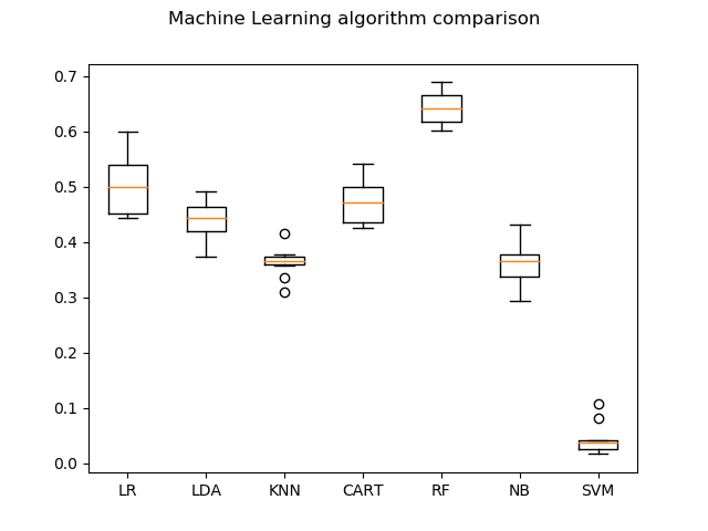
As you can see, the accuracies are not so good. Random Forests (RF) gives the maximum accuracy of 64.38%. This is mainly due to the number of images we use per class. We need large amounts of data to get better accuracy. For example, for a single class, we atleast need around 500-1000 images which is indeed a time-consuming task. But, in this post, I have provided you with the steps, tools and concepts needed to solve an image classification problem.
Testing the best classifier
Let’s quickly try to build a Random Forest model, train it with the training data and test it on some unseen flower images.
train_test.pycode
1
2
3
4
5
6
7
8
9
10
11
12
13
14
15
16
17
18
19
20
21
22
23
24
25
26
27
28
29
30
31
32
33
34
35
36
37
38
39
40
41
42
43
44
45
46
#-----------------------------------
# TESTING OUR MODEL
#-----------------------------------

# to visualize results
import matplotlib.pyplot as plt

# create the model - Random Forests
clf  = RandomForestClassifier(n_estimators=num_trees, random_state=seed)

# fit the training data to the model
clf.fit(trainDataGlobal, trainLabelsGlobal)

# loop through the test images
for file in glob.glob(test_path + "/*.jpg"):
    # read the image
    image = cv2.imread(file)

    # resize the image
    image = cv2.resize(image, fixed_size)

    ####################################
    # Global Feature extraction
    ####################################
    fv_hu_moments = fd_hu_moments(image)
    fv_haralick   = fd_haralick(image)
    fv_histogram  = fd_histogram(image)

    ###################################
    # Concatenate global features
    ###################################
    global_feature = np.hstack([fv_histogram, fv_haralick, fv_hu_moments])

    # scale features in the range (0-1)
    scaler = MinMaxScaler(feature_range=(0, 1))
    rescaled_feature = scaler.fit_transform(global_feature)

    # predict label of test image
    prediction = clf.predict(rescaled_feature.reshape(1,-1))[0]

    # show predicted label on image
    cv2.putText(image, train_labels[prediction], (20,30), cv2.FONT_HERSHEY_SIMPLEX, 1.0, (0,255,255), 3)

    # display the output image
    plt.imshow(cv2.cvtColor(image, cv2.COLOR_BGR2RGB))
    plt.show()
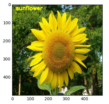
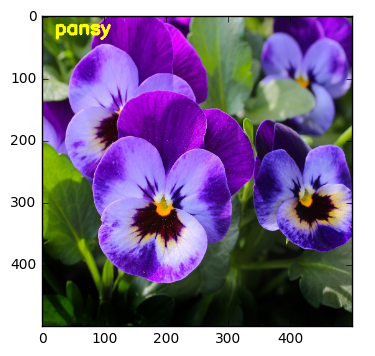
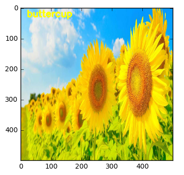
As we can see, our approach seems to do pretty good at recognizing flowers. But it also predicted wrong label like the last one. Instead of sunflower, our model predicted buttercup.
You can download the entire code used in this post here.
Improving classifier accuracy
So, how are we going to improve the accuracy further? Fortunately, there are multiple techniques to achieve better accuracy. Some of them are listed below.
- Gather more data for each class. (500-1000) images per class.
- Use Data Augmentation to generate more images per class.
- Global features along with local features such as SIFT, SURF or DENSE could be used along with Bag of Visual Words (BOVW) technique.
- Local features alone could be tested with BOVW technique.
- Convolutional Neural Networks - State-of-the-art models when it comes to Image Classification and Object Recognition.
Some of the state-of-the-art Deep Learning CNN models are mentioned below.
- AlexNet
- Inception-V3
- Xception
- VGG16
- VGG19
- OverFeat
- ZeilerNet
- MSRA
But to apply CNN to this problem, the size of our dataset must be large enough and also to process those tremendous amount of data it is always recommended to use GPUs.
References
Research Papers
- A Visual Vocabulary for Flower Classification
- Delving into the whorl of flower segmentation
- Automated flower classification over a large number of classes
- Fine-Grained Plant Classification Using Convolutional Neural Networks for Feature Extraction
- Fine-tuning Deep Convolutional Networks for Plant Recognition
- Plant species classification using deep convolutional neural network
- Plant classification using convolutional neural networks
- Deep-plant: Plant identification with convolutional neural networks
- Deep Neural Networks Based Recognition of Plant Diseases by Leaf Image Classification
- Plant Leaf Identification via A Growing Convolution Neural Network with Progressive Sample Learning
Libraries and Tools
Datasets
In case if you found something useful to add to this article or you found a bug in the code or would like to improve some points mentioned, feel free to write it down in the comments. Hope you found something useful here.