When I began to study Neural Networks during my coursework, I realized the complexity involved in representing those large layers of neurons in code. But when I read about Keras and started experimenting with it, everything was super easy to understand and perfectly made sense.
To all those who want to actually write some code to build a Deep Neural Network, but don’t know where to begin, I highly suggest you to visit Keras website as well as it’s github page.
Update: As Python2 faces end of life, the below code only supports Python3.
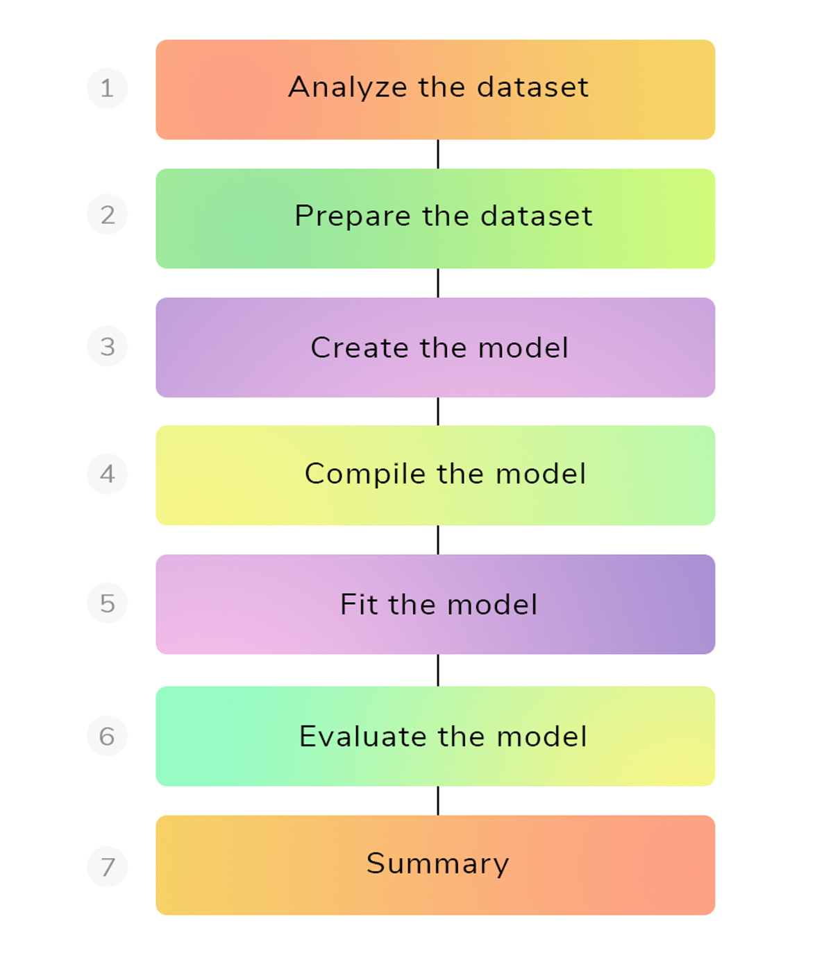
In this post, we will learn the simple 6 steps with which we can create our first deep neural network using Keras and Python. Let’s get started!
1
2
3
4
5
6
7
* How to setup environment to create Deep Neural Nets?
* How to analyze and understand a training dataset?
* How to load and work with .csv file in Python?
* How to work with Keras, NumPy and Python for Deep Learning?
* How to create a Deep Neural Net in less than 5 minutes?
* How to split training and testing data for evaluating our model?
* How to display metrics to analyze performance of our model?
Deep Learning Environment Setup
Before getting into concept and code, we need some libraries to get started with Deep Learning in Python. Copy and paste the below commands line-by-line to install all the dependencies needed for Deep Learning using Keras in Linux. I used Ubuntu 14.04 LTS 64-bit architecture as my OS and I didn’t use any GPU to speed up computations for this tutorial.
1
2
3
4
5
6
7
8
9
10
sudo pip install numpy
sudo pip install scipy
sudo pip install matplotlib
sudo pip install seaborn
sudo pip install scikit-learn
sudo pip install pillow
sudo pip install h5py
sudo pip install --upgrade --no-deps git+git://github.com/Theano/Theano.git
sudo pip install tensorflow
sudo pip install keras
Keras needs Theano or TensorFlow as its backend to perform numerical computations. TensorFlow won’t work in Ubuntu 32-bit architecture (at the time of writing this tutorial). So, better have a 64-bit OS to properly install Keras with both TensorFlow and Theano backend.
If you need to work with Deep Learning on a Windows machine, please visit my post on environment setup for Windows here.
Deep Learning flowchart
Let’s talk about the classic Supervised Learning problem.
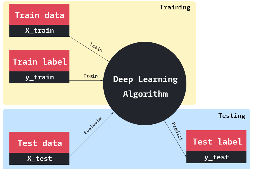
Supervised Learning means we have a set of training data along with its outcomes (classes or real values). We train a deep learning model with the training data so that the model will be in a position to predict the outcome (class or real value) of future unseen data (or test data).
This problem has two sub-divisions namely Classification and Regression.
- Classification - If the output variable to be predicted by our model is a label or a category, then it is a Classification problem. Ex: Predicting the name of a flower species.
- Regression - If the output variable to be predicted by our model is a real or continuous value (integer, float), then it is a Regression problem. Ex: Predicting the stock price of a company.
We will concentrate on a Supervised Learning Classification problem and learn how to implement a Deep Neural Network in code using Keras.
Note: To learn more about Deep Learning theory, I highly suggest you to register in Andrew NG's machine learning course and deep learning course at Coursera or visit Stanford University's awesome website.
Download the below image for your future reference. Any complex problem related to Supervised Learning can be solved using this flowchart. We will walk through each step one-by-one in detail.
Analyse the Dataset
Deep Learning is all about Data and Computational Power.
You read it right! The first step in any Deep Learning problem is to collect more data to work with, analyse the data thoroughly and understand the various parameters/attributes in it. Attributes (also called as features) to look at in any dataset are as follows.
- Dataset characteristics - Multivariate, Univariate, Sequential, Time-series, Text.
- Attribute characteristics - Real, Integers, Strings, Float, Binary.
- Number of Instances - Total number of rows.
- Number of Attributes - Total number of columns.
- Associated Tasks - Classification, Regression, Clustering, Other problem.
For this tutorial, we will use the Pima Indian Diabetes Dataset from Kaggle. This dataset contains the patient medical record data for Pima Indians and tell us whether they had an onset of diabetes within 5 years or not (last column in the dataset). It is typically a binary classification problem where
- 1 = yes! the patient had an onset of diabetes in 5 years.
- 0 = no! the patient had no onset of diabetes in 5 years.
In this dataset, there are 8 attributes (i.e 8 columns) that describes each patient (i.e a single row) and a total of 768 instances (i.e total number of rows or number of patients).
Go to this link, register/login, download the dataset, save it inside a folder named pima-indians-diabetes and rename it as dataset.csv. Below is the folder structure to follow.
1
2
3
|--pima-indians-diabetes
|--|--dataset.csv
|--|--train.py
Prepare the dataset
Data must be represented in a structured way for computers to understand.
Representing our analyzed data is the next step to do in Deep Learning. Data will be represented as an n-dimensional matrix in most of the cases (whether it is numerical or images or videos). Some of the common file-formats to store matrices are csv, cPickle and h5py. If you have millions of data (say millions of images), h5py is the file-format of choice. We will stick with CSV file-format in this tutorial.
CSV (Comma Separated Values) file formats can easily be loaded in Python in two ways. One using NumPy and other using Pandas. We will use NumPy.
Below is the code to import all the necessary libraries and load the pima-indians diabetes dataset.
1
2
3
4
5
6
7
8
9
10
11
12
13
14
15
16
17
18
19
# organize imports
from keras.models import Sequential
from keras.models import Dense
from sklearn.model_selection import train_test_split
import numpy as np

# seed for reproducing same results
seed = 9
np.random.seed(seed)

# load pima indians dataset
dataset = np.loadtxt('dataset.csv', delimiter=',', skiprows=1)

# split into input and output variables
X = dataset[:,0:8]
Y = dataset[:,8]

# split the data into training (67%) and testing (33%)
(X_train, X_test, Y_train, Y_test) = train_test_split(X, Y, test_size=0.33, random_state=seed)
- Line (1-3) handles the imports to build our deep learning model using Keras.
- Line (6-7) fix a seed for reproducing same results if we wish to train and evaluate our network more than once.
- Line (10) loads the dataset from the .csv file saved on disk. It uses an argument delimiter to inform NumPy that all attributes are separated by , in the .csv file.
- Line (13-14) splits the dataset into input and output variables.
- X has all the 8 attributes of the patients
- Y has whether they have an onset of diabetes or not.
- Line (17) splits the dataset into training (67%) and testing (33%) using the scikit-learn’s train_test_split function. By performing this split, we can easily verify the performance of our model in an unseen test dataset.
Create the Model
In Keras, a model is created using Sequential. You may wanna recall that Neural Networks holds large number of neurons residing inside several sequential layers.
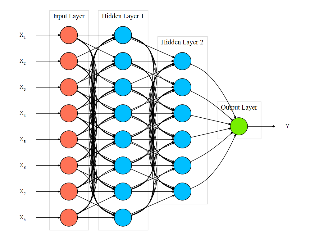
We will create a model that has fully connected layers, which means all the neurons are connected from one layer to its next layer. This is achieved in Keras with the help of Dense function.
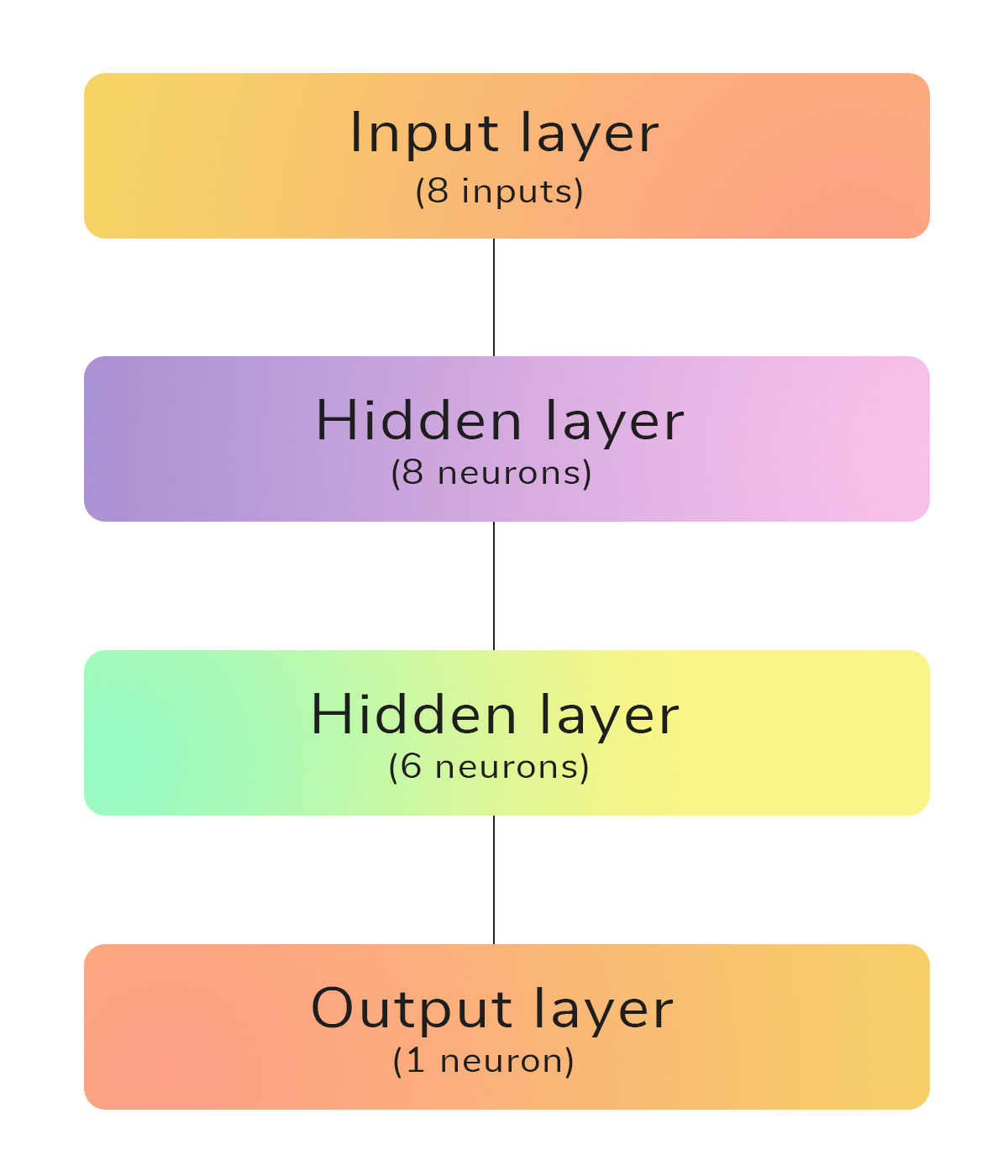
We will use the above Deep Neural Network architecture which has a single input layer, 2 hidden layers and a single output layer.
The input data which is of size 8 is sent to the first hidden layer that has randomly initialized 8 neurons. This is a very useful approach, if we don’t have any clue about the no.of.neurons to specify at the very first attempt. From here, we can easily perform trial-and-error procedure to increase the network architecture to produce good results. The next hidden layer has 6 neurons and the final output layer has 1 neuron that outputs whether the patient has an onset of diabetes or not.
Figure 4 shows our Deep Neural Network with an input layer, a hidden layer having 8 neurons, a hidden layer having 6 neurons and an output layer with a single neuron.
Below are the four lines of code to create the above architecture.
1
2
3
4
5
# create the model
model = Sequential()
model.add(Dense(8, input_dim=8, init='uniform', activation='relu'))
model.add(Dense(6, init='uniform', activation='relu'))
model.add(Dense(1, init='uniform', activation='sigmoid'))
- Line (1) creates a Sequential model to add layers one at a time.
- Line (2), the first layer expects four arguments:
- 8: No.of.neurons present in that layer.
- input_dim: specify the dimension of the input data.
- init: specify whether uniform or normal distribution of weights to be initialized.
- activation: specify whether relu or sigmoid or tanh activation function to be used for each neuron in that layer.
- Line (3), the next hidden layer has 6 neurons with an uniform initialization of weights and relu activation function
- Line (4), the output layer has only one neuron as this is a binary classification problem. The activation function at output is sigmoid because it outputs a probability in the range 0 and 1 so that we could easily discriminate output by assigning a threshold.
Compile the model
After creating the model, three parameters are needed to compile the model in Keras.
- loss: This is used to evaluate a set of weights. It is needed to reduce the error between actual output and expected output. It could be binary_crossentropy or categorical_crossentropy depending on the problem. As we are dealing with a binary classification problem, we need to pick binary_crossentropy. Here is the list of loss functions available in Keras.
- optimizer: This is used to search through different weights for the network. It could be adam or rmsprop depending on the problem. Here is the list of optimizers available in Keras.
- metrics: This is used to collect the report during training. Normally, we pick accuracy as our performance metric. Here is the list of metrics available in Keras.
These parameters are to be tuned according to the problem as our model needs some optimization in the background (which is taken care by Theano or TensorFlow) so that it learns from the data during each epoch (which means reducing the error between actual output and predicted output).
epoch is the term used to denote the number of iterations involved during the training process of a neural network.
1
2
# compile the model
model.compile(loss='binary_crossentropy', optimizer='adam', metrics=['accuracy'])
- Line (2) chooses a binary_crossentropy loss function and the famous Stochastic Gradient Descent (SGD) optimizer adam. It also collects the accuracy metric for training.
Fit the model
After compiling the model, the dataset must be fitted with the model. The fit() function in Keras expects five arguments -
- X_train: the input training data.
- Y_train: the output training classes.
- validation_data: Tuple of testing or validation data used to check the performance of our network.
- nb_epoch: how much iterations should the training process take place.
- batch_size: No.of.instances that are evaluated before performing a weight update in the network.
1
2
# fit the model
model.fit(X_train, Y_train, validation_data=(X_test, Y_test), nb_epoch=100, batch_size=5)
- Line (2) chooses 100 iterations to be performed by the deep neural network with a batch_size of 5.
Evaluate the model
After fitting the dataset to the model, the model needs to be evaluated. Evaluating the trained model with an unseen test dataset shows how our model predicts output on unseen data. The evaluate() function in Keras expects two arguments.
- X - the input data.
- Y - the output data.
1
2
3
# evaluate the model
scores = model.evaluate(X_test, Y_test)
print("Accuracy: %.2f%%" %(scores[1]*100))
Complete code
Excluding comments and empty new lines, we have combined all the 6 steps together and created our first Deep Neural Network model using 18 lines of code. Below is the entire code of the model we have just built.
1
2
3
4
5
6
7
8
9
10
11
12
13
14
15
16
17
18
19
20
21
22
23
24
25
26
27
28
29
30
31
32
33
34
35
# organize imports
from keras.models import Sequential
from keras.layers import Dense
from sklearn.model_selection import train_test_split
import numpy as np

# seed for reproducing same results
seed = 9
np.random.seed(seed)

# load pima indians dataset
dataset = np.loadtxt('dataset.csv', delimiter=',', skiprows=1)

# split into input and output variables
X = dataset[:,0:8]
Y = dataset[:,8]

# split the data into training (67%) and testing (33%)
(X_train, X_test, Y_train, Y_test) = train_test_split(X, Y, test_size=0.33, random_state=seed)

# create the model
model = Sequential()
model.add(Dense(8, input_dim=8, init='uniform', activation='relu'))
model.add(Dense(6, init='uniform', activation='relu'))
model.add(Dense(1, init='uniform', activation='sigmoid'))

# compile the model
model.compile(loss='binary_crossentropy', optimizer='adam', metrics=['accuracy'])

# fit the model
model.fit(X_train, Y_train, validation_data=(X_test, Y_test), nb_epoch=200, batch_size=5, verbose=0)

# evaluate the model
scores = model.evaluate(X_test, Y_test)
print("Accuracy: %.2f%%" % (scores[1]*100))
- Save the code with a filename train.py in the same folder as the dataset.
- Open up a command prompt and go to that folder.
- Type python train.py
I got an accuracy of 72.83% which is pretty good in our first try without any hyperparameter tuning or changing the network architecture.
Kindly post your results in the comments after tuning around with nb_epoch, batch_size, activation, init, optimizer and loss. You can also increase the number of hidden layers and the number of neurons in each hidden layer.
Summary
Thus, we have built our first Deep Neural Network (Multi-layer Perceptron) using Keras and Python in a matter of minutes. Note that we haven’t even touched any math involved behind these Deep Neural Networks as it needs a separate post to understand. We have strictly focused on how to solve a supervised learning classification problem using Keras and Python.
In case if you found something useful to add to this article or you found a bug in the code or would like to improve some points mentioned, feel free to write it down in the comments. Hope you found something useful here.